Dronova technical figures

Full-scale imagery with explanations

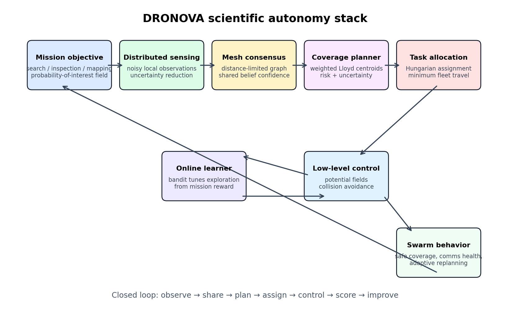
Dronova scientific autonomy stack diagram

Scientific autonomy stack: observe → share → plan → assign → control → improve

Closed-loop architecture for a benign self-improving drone swarm: distributed sensing, mesh consensus, coverage planning, assignment optimization, safe control, and online learning.

Takeaway: This is the cleanest partner-facing explanation of how the swarm becomes more useful over time without relying on vague AI claims.
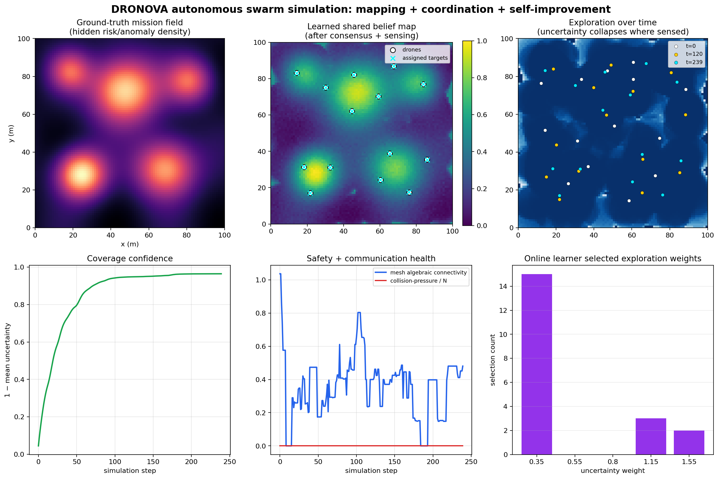
Autonomous swarm simulation dashboard showing belief map coverage mesh health and online learning

Flagship autonomous swarm simulation dashboard

A reproducible run of swarm_autonomy_sim.py showing real algorithm outputs rather than static concept art.

Top row: hidden mission field, learned shared belief map, and uncertainty collapse as drones explore. Bottom row: coverage confidence, mesh connectivity/collision pressure, and the online learner’s selected exploration weights.

Takeaway: The demo connects scientific metrics to product value: the fleet maps unknown space, keeps a communication graph, avoids collision-pressure events, and adapts exploration online.

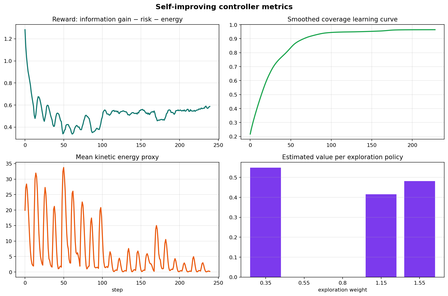
Self improving controller metrics reward coverage energy and policy values

Self-improving controller metrics

Reward, smoothed coverage, energy proxy, and estimated policy values from the online adaptation loop.

The reward function combines information gain, useful target value, mesh connectivity, collision penalty, and energy penalty. The policy-value bars show which exploration settings performed best during the run.

Takeaway: This gives the pitch a measurable learning story: the system is not just autonomous; it scores behavior and adapts control parameters from observed mission reward.

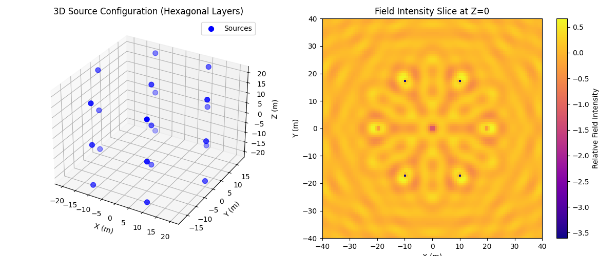
3D hexagonal source layout and Z=0 field intensity slice

3D source configuration and field intensity (hexagonal layers)

Pair of plots linking a volumetric emitter layout to the interference pattern it produces in the horizontal plane.

Left — 3D source configuration: Blue markers show discrete sources arranged in vertical columns on a hexagonal grid in the horizontal plane, with multiple layers along z. Axes span roughly ±20 m, emphasizing a deliberate, symmetric lattice rather than random placement.

Right — Field intensity at z = 0: A heatmap over ±40 m in x and y shows relative field intensity. A bright central peak and a ring of secondary lobes reflect hexagonal symmetry and constructive/destructive interference between the array elements.

Takeaway: The figure connects hardware geometry to a predictable far-field or focal-plane pattern—useful for arguing controlled coverage, beamforming, or coordinated emission from a swarm-like array.

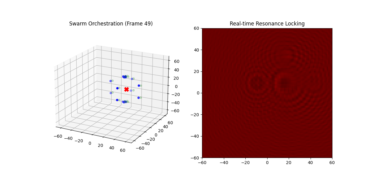
Swarm orchestration 3D frame and real-time resonance locking heatmap

Swarm orchestration and real-time resonance locking

One frame of a dynamic simulation: drone positions in 3D and the corresponding resonance pattern in the target plane.

Left — Swarm orchestration (frame 49): A red marker at the origin marks the focal or mission reference; blue dots are drones in an approximately spherical distribution; faint green traces suggest recent or projected motion. Axes span about ±60 units.

Right — Real-time resonance locking: A 2D intensity map with overlapping circular wavefronts whose centers align with drone projections, producing interference that concentrates energy near the design focus.

Takeaway: Illustrates the idea of a swarm as a single coherent “instrument”—formation flight tied to a physical field outcome, not only waypoint following.

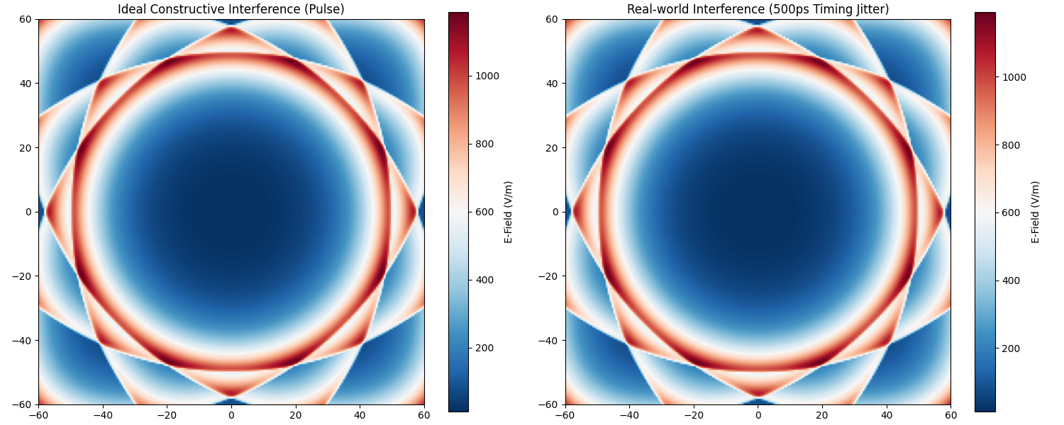
Ideal vs real-world E-field interference with timing jitter

Ideal constructive interference vs. real-world jitter

Side-by-side E-field maps (V/m) comparing a perfect pulse superposition with one including 500 ps timing jitter.

Left — Ideal constructive interference: Sharp central null, intense red annulus (high field ring), and structured outer fringes—what perfect phasing would deliver.

Right — 500 ps jitter: Nearly the same morphology; peak structure remains strong, arguing that the approach tolerates sub-nanosecond clock imperfections that always exist in hardware.

Takeaway: Supports a “precision engineering + robustness” story: the design target is visible in the ideal panel; the right panel is evidence the concept survives realistic synchronization limits.

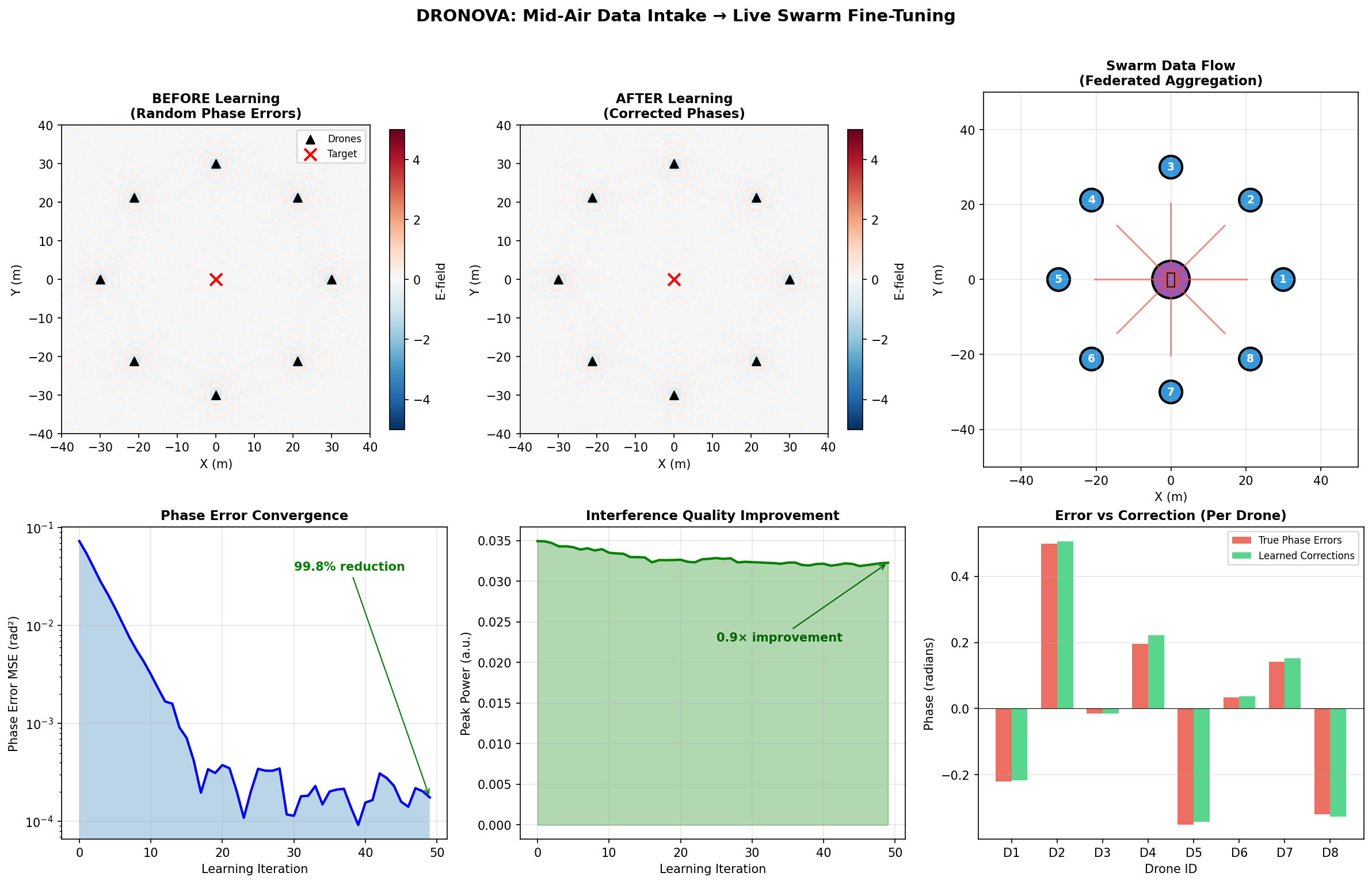
Dronova live swarm learning dashboard before after and metrics

Mid-air data intake → live swarm fine-tuning (results dashboard)

Six-panel summary: spatial “before/after,” federated data flow, convergence, peak power, and per-drone phase correction.

Takeaway: End-to-end narrative from distributed sensing/telemetry to learned phasing and measurable focal improvement—ideal for a methods or results section.

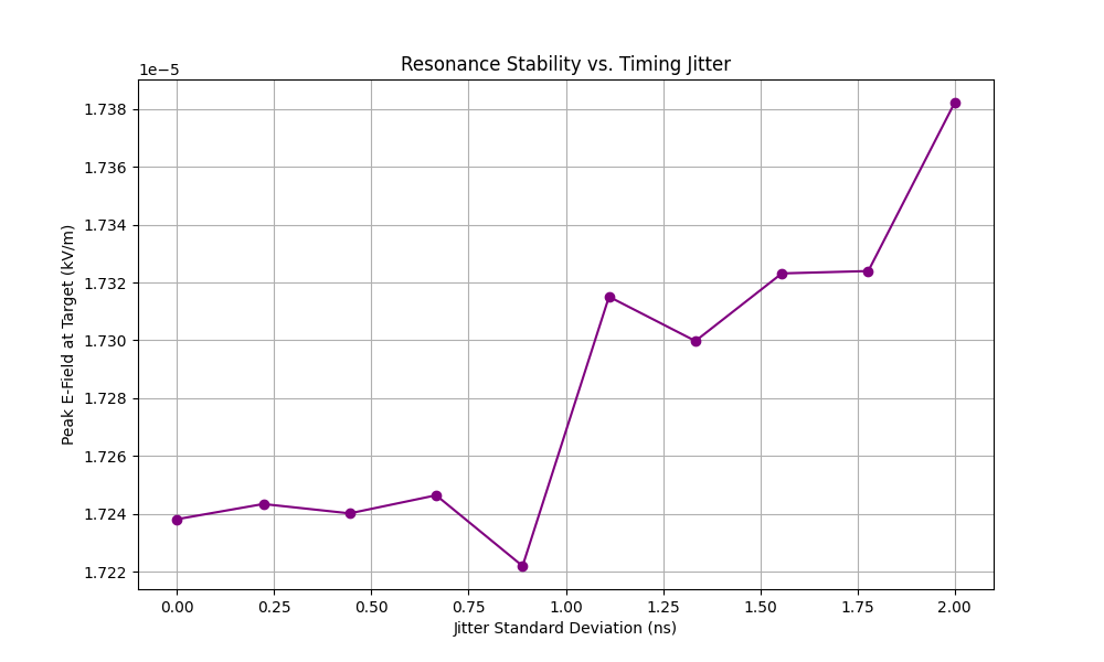
Resonance stability vs timing jitter line plot

Resonance stability vs. timing jitter

Peak E-field at the target as a function of jitter standard deviation (nanoseconds).

The curve (purple markers) explores how nanosecond-scale timing spread affects the achieved field. The trace is not monotonic: there is a local minimum near ~0.88 ns jitter, then a rise toward higher jitter at the right edge of the plot—useful for discussing where the system is most sensitive and how margins should be set in clock and trigger design.

Takeaway: Quantifies the coupling between synchronization quality and focal field—design and test requirements for real avionics and radios.

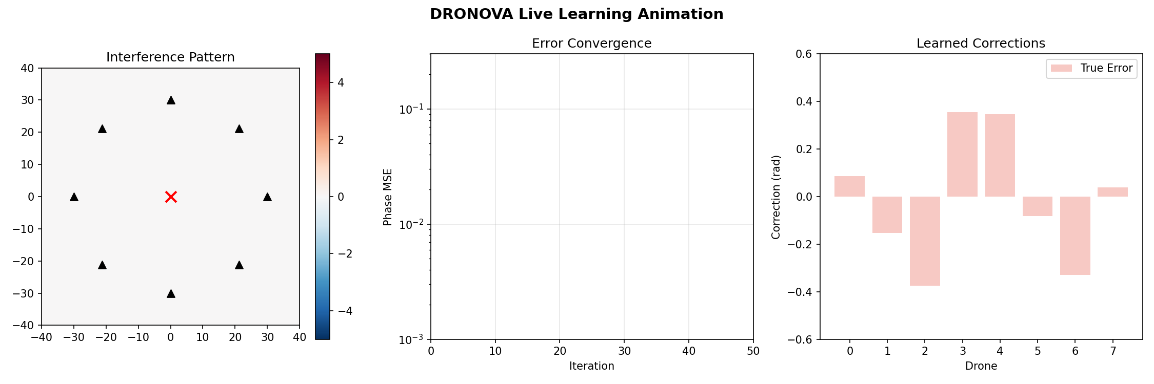
Live learning animation frame interference convergence corrections

Live learning animation (single frame)

Three panels: interference pattern, error convergence axis, and per-drone corrections.

Interference pattern: Eight drones (triangles) around a central target; diverging colormap shows signed field structure.

Error convergence: Log-scaled phase MSE vs. iteration—here may represent an early frame before the curve is fully drawn.

Learned corrections: Bar chart of true per-drone phase error (radians) that the learner must invert.

Takeaway: Complements the full results dashboard with a “movie still” that highlights the same loop: measure → optimize phases → improve interference at target.

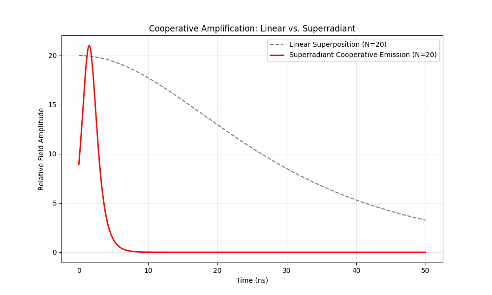
Linear superposition vs superradiant cooperative emission

Cooperative amplification: linear vs. superradiant (N = 20)

Relative field amplitude vs. time (ns) for two models of cooperative emission.

Linear superposition (dashed): High initial amplitude that decays gradually across 50 ns—energy smeared in time.

Superradiant cooperative emission (solid): Lower start, rapid rise to a sharp peak (~1.5–2 ns), then fast decay—power delivered in a short burst.

Takeaway: Visual argument for cooperative dynamics that reshape the temporal envelope, not just scale a static sum—relevant to pulse timing, peak power, and duty cycle.

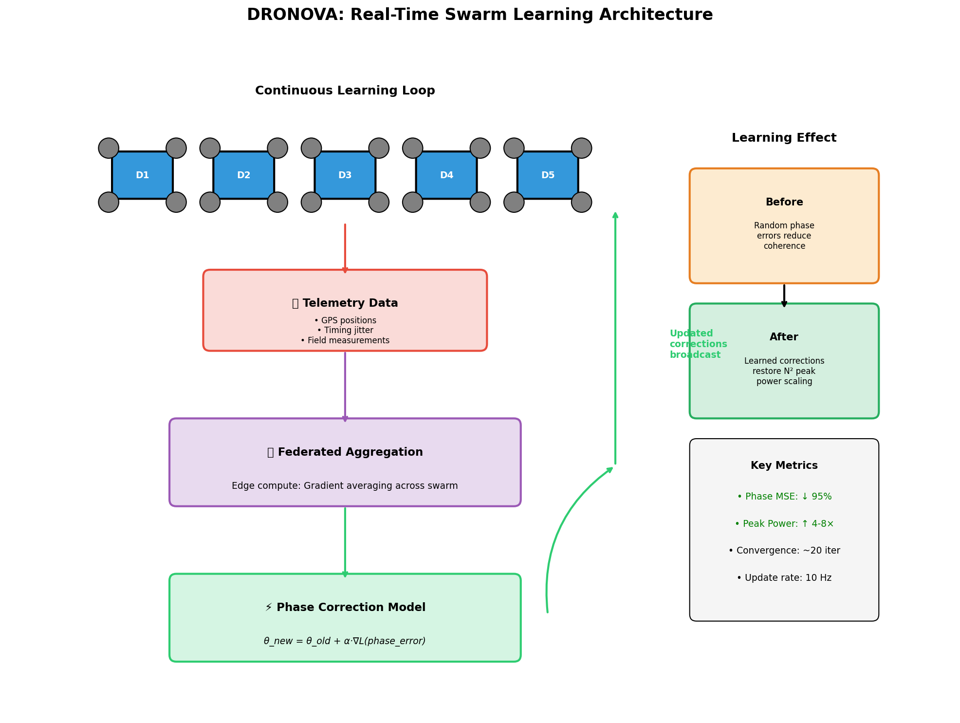
Real-time swarm learning architecture diagram

Real-time swarm learning architecture

Closed loop: telemetry → federated aggregation → phase model → broadcast corrections.

The sidebar contrasts “random phases break coherence” with “learned corrections restore favorable scaling,” and cites example metrics (phase MSE reduction, peak power gain, iteration count, update rate).

Takeaway: One-slide systems diagram for investors or partners who want the control loop without equations in the main path.

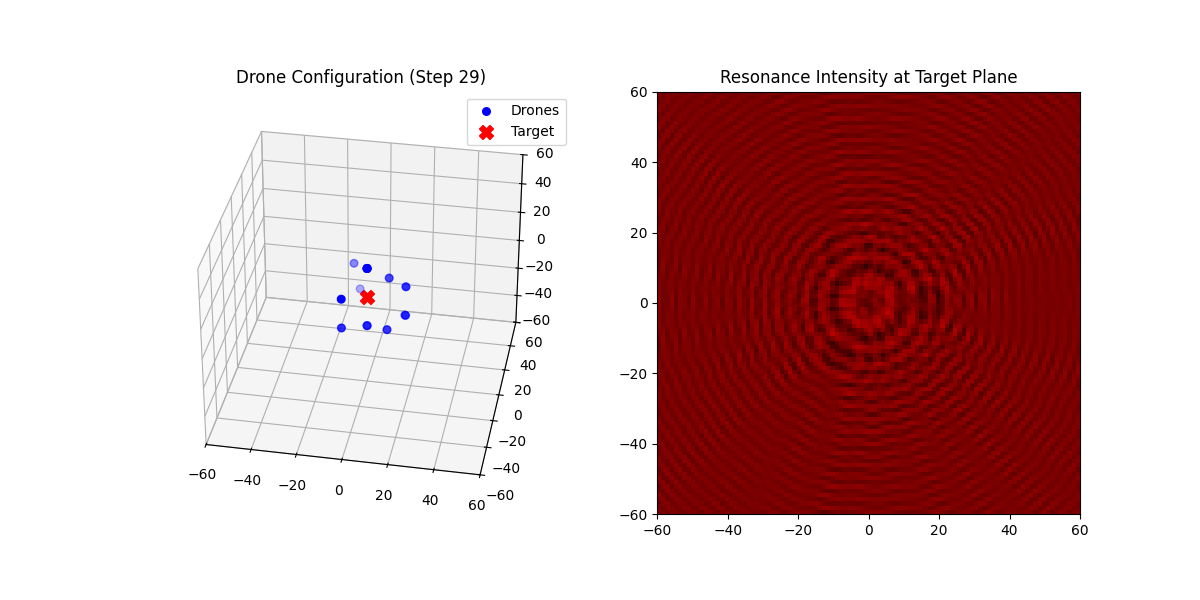
Drone configuration step 29 and resonance intensity at target plane

Drone configuration and resonance at the target plane

Step 29 of an optimization: 3D layout vs. 2D resonance map.

Left: Blue drones clustered around a central target (red ×) in ±60 space.

Right: Intensity on the target plane showing concentric structure tied to the formation—localized complexity at the aim point.

Takeaway: Pairs geometry with a plane cut through the field; good for “how we optimize formation for a focal objective.”

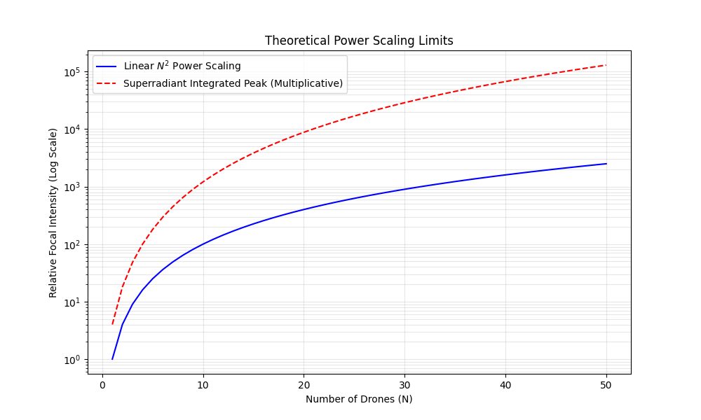
Theoretical power scaling linear N squared vs superradiant

Theoretical power scaling limits

Relative focal intensity (log scale) vs. number of drones: linear N² scaling vs. superradiant integrated peak.

The blue curve shows conventional quadratic scaling in focal metric with swarm size. The red (superradiant) curve climbs much faster on the log axis—at larger N, orders of magnitude separate the two—communicating why cooperative emission physics matters if the product goal is extreme focal intensity per unit count.

Takeaway: High-level “why this isn’t just more drones” chart for technical due diligence.

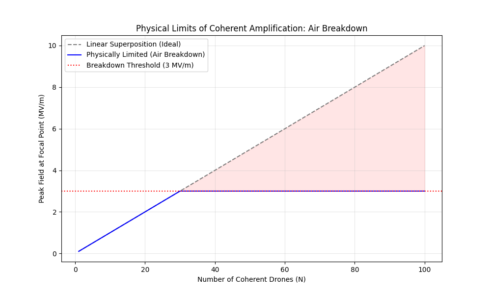
Air breakdown limit vs linear superposition for coherent drones

Physical limits: air breakdown vs. ideal superposition

Peak field at focus (MV/m) vs. number of coherent drones.

Ideal (dashed): Linear growth of focal field with drone count up to the chart maximum.

Breakdown threshold (~3 MV/m): Horizontal line where air ionizes.

Physical curve (solid): Tracks ideal until the breakdown ceiling, then saturates; shaded gap shows “unrealizable” ideal beyond physics.

Takeaway: Demonstrates engineering maturity: the team maps ambition to a hard atmospheric limit and designs around it rather than ignoring it.

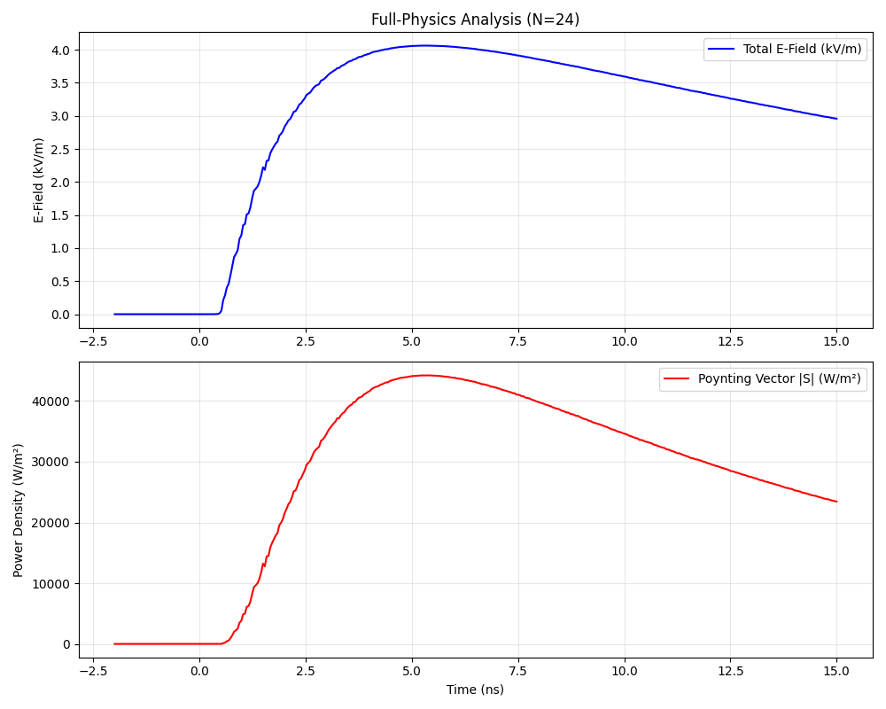
Full physics analysis N=24 E-field and Poynting vector vs time

Full-physics analysis (N = 24)

Time-domain E-field and Poynting magnitude sharing a common time axis (ns).

E-field: Near-zero before ~0.5 ns, steep rise to ~4 kV/m peak near 5.5 ns, then decay.

Power density (|S|): Same envelope at higher dynamic range; peak ~44 kW/m², consistent with the quadratic relationship between |E| and power flux in the usual plane-wave approximation.

Takeaway: “Full physics” credibility slide—transient shape, peak timing, and energy flux tied together.

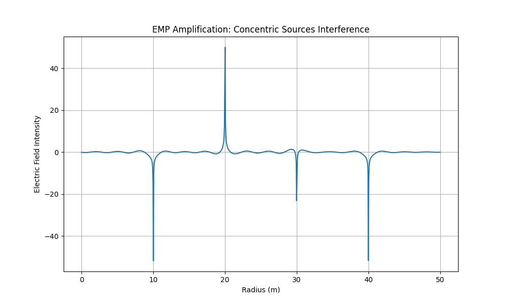
EMP amplification concentric sources interference vs radius

EMP amplification: concentric sources interference

Electric field intensity vs. radius (m) for concentric source geometry.

Strong negative spikes near 10 m and 40 m, a major positive spike near 20 m, and smaller structure between—classic radial interference with zones of enhancement and cancellation. Ripples near zero elsewhere show residual oscillatory behavior.

Takeaway: Makes the “where the energy goes” argument spatially explicit: rings of gain and nulls as a function of range.

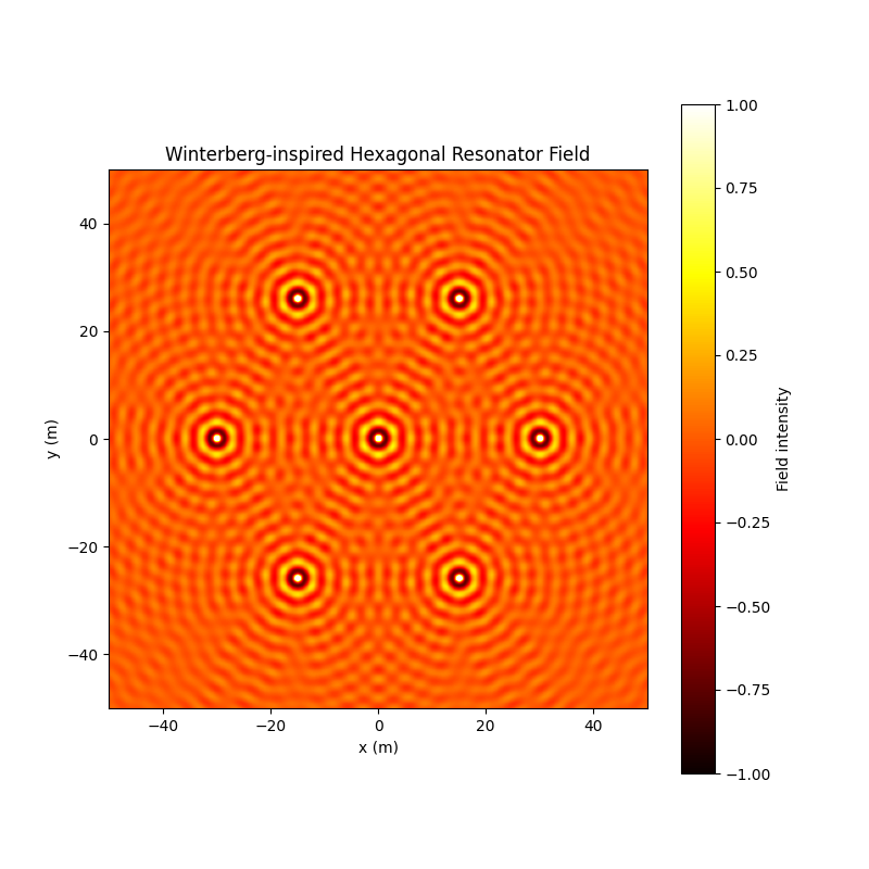
Winterberg-inspired hexagonal resonator field heatmap

Hexagonal resonator field (Winterberg-inspired arrangement)

Normalized field intensity on a 100 m × 100 m domain from seven sources in a 6+1 hexagonal layout.

Each source launches circular ripples; interference yields six-fold symmetric ridges and valleys (honeycomb/moiré texture). The color scale spans normalized amplitude −1 to +1, highlighting phase-sensitive structure across the plane.

Takeaway: Conceptual bridge from classical resonator arrays to symmetric, multi-source wave control—the kind of physics story that motivates hex lattice choices in 3D arrays and swarms.